Flux queries
This page contains Flux queries for displaying various information from the tables. It focuses on the raw_data
table, as the others are trivial to work with.
Grafana workarounds, InfluxQL vs. Flux
Grafanas Flux support is still being worked on, and as such the comfort of using it with Flux is not on-par with the
InfluxQL support yet. The main problem that this page is working around is the inability to remap label names easily in
Grafana. This was done in InfluxQL by using GROUP BY tag(columnname) in the query and $_tag_columname in the
ALIAS BY field of the query wizard. Here, for measurements that are similar to normal tables (they are pre-procesed by
RctMon and contain sensible field names) a simple, beautifying rename() is used.
But for the raw_data measurement, things are more complicated. The measurement uses tags to give meaning to the
fields (of which there are a few, such as value_float or value_string). So in order to query the AC voltage of
Line 1 to 3, the query needs to first filter the measurement to only include the value rows whose name is
g_sync.u_l_rms[0] through [2] and then apply a mapping that changes the name from g_sync.u_l_rms[0] to
L1 and so on.
Hint
This is only a quick introduction to Flux. For the complete set, head over to the Get started with Flux page over at influxdata.com.
It's easier to just use a query as an example. In the example, the bucket is named rct-inverter and the inverter
itself is named PS 6.0 ASDF. If you use only one inverter you may can omit filtering for the inverter name. Flux
works by reading from a data source (from()) and then passing the tabular data through a set of functions, like a
UNIX pipe.
from(bucket: "rct-inverter")
// limit the time range (values from calling application, e.g. Grafana date-picker)
|> range(start: v.timeRangeStart, stop: v.timeRangeStop)
// narrow down the data we want
|> filter(fn: (r) => r._measurement == "raw_data" and r._field == "value_float" and r.inverter == "PS 6.0 ASDF")
// select the metrics we want
|> filter(fn: (r) => r.name == "g_sync.u_l_rms[2]" or r.name == "g_sync.u_l_rms[1]" or r.name == "g_sync.u_l_rms[0]")
// rename metrics to enable "nice" label names in Grafana using Display Name "${__field.labels.name}"
|> map(fn: (r) => ({
r with name:
if r.name == "g_sync.u_l_rms[0]" then "L1"
else if r.name == "g_sync.u_l_rms[1]" then "L2"
else "L3"
}))
// aggregate into time buckets
|> aggregateWindow(every: v.windowPeriod, fn: mean, createEmpty: false)
// return the result
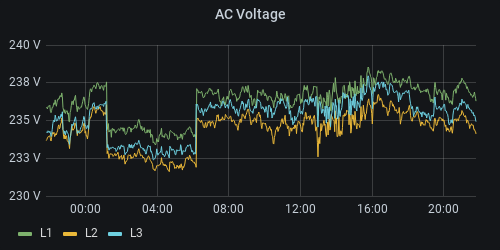
|> yield(name: "AC Voltage")
Let's look at the parts line-by-line:
from(bucket: "rct-inverter")states that it should read from the bucketrct-inverter. This is the same name as set in the configuration, so this value may need adjustment depending on how the user set up their system.|> range(start: v.timeRangeStart, stop: v.timeRangeStop)reduces the data to the time range. The variablevcontains values from the calling system, in this case passed to Flux from the Grafana Date picker (or the date picker in the InfluxDB Data Explorer).|> filter(fn: (r) => r._measurement == "raw_data" and r._field == "value_float" and r.inverter == "PS 6.0 ASDF")is the first filter that reduces the table by only letting rows pass on to the next line if the criteria matches. In this example, the measurement name (aka table name) must beraw_data, and the field we want isvalue_floatfor the voltage is a floating point value. Additonally, it limits by inverter name, which could be omitted if there's only one inverter (and thus one instance of RctMon) in use. This works by defining a function that is called for each row (hence the variable namer) that is passed to it.rcontains all the tags and fields.|> filter(fn: (r) => r.name == "g_sync.u_l_rms[2]" or r.name == "g_sync.u_l_rms[1]" or r.name == "g_sync.u_l_rms[0]")further filters the data, by only passing on the three metrics we want, AC line voltage for the three phases.|> map(fn: (r) => ({ ... })defines a mapping of data. Each row that is processed is subject to the mapping in its body:r with name:is a fancy way of saying: Return the row as-is but change thenameattribute as follows. Without this, each of the rows attributes would need to be mapped manually (input-name → output-name, input-value → output-value and so on).if r.name == "g_sync.u_l_rms[0]" then "L1""returns""L1"if the rowsnameattribute matches. With the previous line stating that it is working on thenameattribute,"L1" is assigned to thenameattribute of the currently proccessed row. The if-statement can work with all the attributes ofr, it is not limited toname.else if r.name == "g_sync.u_l_rms[1]" then "L2"andelse "L3"complete the mapping.
|> aggregateWindow(every: v.windowPeriod, fn: mean, createEmpty: false)aggregates the window into the specified time window.|> yield(name: "AC Voltage")"returns" the data to the caller (Grafana). The name may be omitted if this is the only query that is run. Since Flux can yield more than one result in a single script, it is better to give it a meaningful name all the time. At the minimum, it helps you remember what it does when you look at it at a later point in time.
The result should look similar to this:
Query examples
All of the following examples query from the raw_data measurement and assume that the bucket is named
rct-inverter.
String voltage
from(bucket: "rct-inverter")
    |> range(start: v.timeRangeStart, stop: v.timeRangeStop)
    |> filter(fn: (r) => r._measurement == "raw_data" and r._field == "value_float" and r.inverter == "PS 6.0 ASDF")
    |> filter(fn: (r) => r.name == "g_sync.u_sg_avg[0]" or r.name == "g_sync.u_sg_avg[1]")
    |> map(fn: (r) => ({
        r with name:
            if r.name == "g_sync.u_sg_avg[0]" then "A"
            else "B"
       }))
    |> aggregateWindow(every: v.windowPeriod, fn: mean, createEmpty: false)
    |> yield(name: "DC Voltage")

Battery charge state and charge target
from(bucket: "rct-inverter")
|> range(start: v.timeRangeStart, stop: v.timeRangeStop)
|> filter(fn: (r) => r._measurement == "raw_data" and r._field == "value_float" and r.inverter == "PS 6.0 ASDF")
|> filter(fn: (r) => r.name == "battery.soc" or r.name == "battery.soc_target")
|> map(fn: (r) => ({
r with name:
if r.name == "battery.soc" then "Charge"
else "Target"
}))
|> aggregateWindow(every: v.windowPeriod, fn: mean, createEmpty: false)
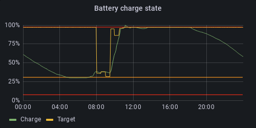
|> yield(name: "Battery Charge")
The following gallery displays a few different widgets, all of them support the visual indication of values via a change in color, except the basic graph panel which uses marker lines. All thresholds are identical: below 7% and above 97% is red, between 30% and 7% yellow is used (between "Min SOC target" and "Min SOC target (island)"), and the middle section is green. These values can't be read from the database automatically, so they must be manually set for the setup at hand.
Graph / Timeseries |
Bar gauge |
|
|---|---|---|
|

|
|
Gauge |
Stat |
|

|

|
|
System and battery temperatures
from(bucket: "rct-inverter")
|> range(start: v.timeRangeStart, stop: v.timeRangeStop)
|> filter(fn: (r) => r._measurement == "raw_data" and r._field == "value_float" and r.inverter == "PS 6.0 ASDF")
|> filter(fn: (r) => r.name == "battery.temperature" or r.name == "db.temp1" or r.name == "db.temp2" or r.name == "db.core_temp")
|> map(fn: (r) => ({
r with name:
if r.name == "battery.temperature" then "Battery"
else if r.name == "db.temp1" then "Temp1"
else if r.name == "db.temp2" then "Temp2"
else "Core"
}))
|> aggregateWindow(every: v.windowPeriod, fn: mean, createEmpty: false)
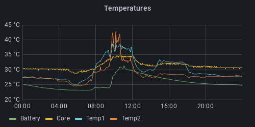
|> yield(name: "Temperatures")
Inverter status
The status is encoded as an integer value that must be mapped to something more useful.
from(bucket: "rct-inverter")
    |> range(start: v.timeRangeStart, stop: v.timeRangeStop)
    |> filter(fn: (r) => r._measurement == "raw_data" and r._field == "value_int" and r.inverter == "PS 6.0 ASDF" and r.name == "prim_sm.state")
    |> aggregateWindow(every: v.windowPeriod, fn: max, createEmpty: false)
    |> yield(name: "Inverter Status")
The mapping is as follows:
State |
Name |
|---|---|
0 |
Standby |
1 |
Initialization |
2 |
Standby |
3 |
Efficiency |
4 |
Insulation check |
5 |
Island check |
6 |
Power check |
7 |
Symmetry |
8 |
Relais test |
9 |
Grid passive |
10 |
Prepare Bat Passive |
11 |
Battery Passive |
12 |
H/W check |
13 |
Feed in |
In a typical environment, the states that will be encountered are:
13 / Feed in: This is the desired state, meaning that there is enough power from solar generators and/or battery.
6 / Power check: This state is encountered when there is not enough input power, meaning no sunlight and the batteries State of charge (
battery.soc) is at or below the value of Min SOC target (power_mng.soc_min). Note that if the battery reaches the value set in Min SOC target (island) (power_mng.soc_min_island) the battery will shut off, and if the solar generators are not producing power then the device will power off completely, and can't be reached over the network until input power is restored (usually sunrise).5 / Island check: The state is briefly encountered when transitioning from Feed in to Power check.
7 / Symmetry: The state is briefly encountered when transitioning from Power check to Feed in:
One way to visualise this is to use the natel-discrete-panel that can be found on Grafana.com:
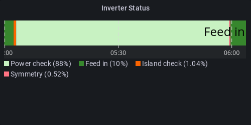
Another option is to use the new "State timeline" panel type that is new in Grafana 8:
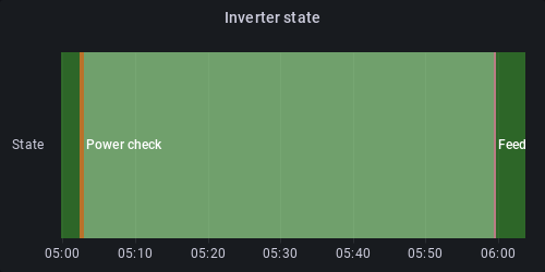
Both of these have their strengths and weaknesses, and some experimentation may be required to get the most out of them.